The Financial Implications of Order Lead Times, Order Frequency, and JIT for Distributors

Some suppliers offer “Just in Time” (JIT) inventory and delivery programs as benefit to their customers. They can do this if they have managed to get their own inventory situations under tighter control. This situation can be a boon to you, the distributor, providing that you have a full understanding of the implications of better delivery programs, and you have the systems in place to take advantage of these opportunities. Additionally, the suppliers will often want a slight price increase (and hence a lower gross margin to you) in return for this better service, making the need to capitalize on these programs that much more critical.
Simulations
We ran a series of simulations to explore this issue further, which are summarized in the tables below. To simplify the simulation, we are using a relatively flat, non-seasonal demand projection. The same concepts can be applied to variable demand and seasonal items.
The product used in the example has the following characteristics:
- Monthly sales volume: 400 units
- Mean Average Deviation (MAD*): 50
- Cost: $30/Unit
- Desired Fill Rate: 95%
*MAD is a measure of demand variability. It predicts the volatility of your demand forecast and is used to calculate safety stock coverage amongst other things. We’ll cover MAD in depth in a later whitepaper. In this case we use a MAD of 50 which means the item has fair, but not great predictability.
Summary of Various Simulations of Inventory Needed
The above tables display the inventory needed strictly to meet the 95% fill rate, and does not consider lot sizing, pallet requirements, Economic Order Quantity (EOQ) considerations, discounts being taken, etc. It also says nothing about the dead stock which constitutes from 20 to 40% of most distributors inventory. Moreover, it assumes the use of an Inventory Replenishment system such as Mars Inventory Workstation with its strong reorder point calculations (yes, we are going to plug our product – but the simulation would be valid using a competitive product as well).
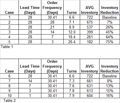
For our baseline, we will assume that you order 12 times a year (on average every 30.41 days) and the lead time is 28 days. Lead time includes your acquisition time, transit time and receiving. All of the time between generating a requisition and having stock on hand to ship to customers. Selling an average of 400 units a month, the average stock on hand would be around 722 units.
Table 1 shows the effect of increasing the order frequency without reducing the lead time. Just ordering 13 times a year – every four weeks – decreases the average inventory by 7%. At $30/unit that is a savings of $1500/month while maintaining our 95% fill rate! Order every week, even with a 28 day lead time and you reduce your average inventory by 64%.
Table 2 shows the effect of reducing the lead time without increasing the order frequency. Certainly you reduce your average inventory by getting the product faster (shortening your exposure period). But the reduction in inventory peaks at 15% with only a 3 day total lead time.
Conclusions
Consequently, it is the relative performance between the examples that is pertinent for this discussion. The most significant impact you can make to decrease your average inventory without putting your desired fill rate at risk relates to the order frequency. Note how the amount of inventory needed responds much more aggressively to the reduction in order frequency than to lead time. This phenomena is very logical, since, as the frequency of reordering is increased, most of the product is driven into the pipeline, whereas lead time actually means the product arrives faster and spends more time in your warehouse.
All of this analysis and discussion is academic however, unless you are using an inventory management system that will optimize the opportunities that are being offered to you. Manual reordering, aided only with spreadsheets that must be visually scanned, can make only some “gut feel” improvement, and will certainly fail to drive the inventory back into the pipeline. Simplistic systems, with their weak reorder point calculations and safety stock determinations will also fail to capitalize on the new opportunities.
The need to take advantage of the improved lead times and order frequency becomes particularly apparent when you consider the economic implications of giving up gross margin to the vendor. If we use the above example, where the product costs $30 a unit and moves at 400 units per month, a drop of 1% point is worth $120/ month in gross margin loss. To offset just this 1% drop in gross margin we would have to drop inventories of that item by 267 units (assuming an 18% carrying cost of inventory). That is greater than the full spread between the best and worst case lead time reduction examples above.
On the other hand, if the above example were managed by a manual or simplistic system, you would be getting about 4 to 7 turns (if you were lucky) which equates to having about 700 to 1000 units in inventory. Now we are talking about a realistic expected reduction of at least 200 units, if not 400 to 500 under the most aggressive of circumstances.
The Bottom Line
Even without a vendor offering a JIT program, moving from a manual or simplistic system to a strong MARS type system that can support a 7 day reorder cycle can provide inventory reductions that equate to several points of gross margin (something management would be willing to kill for in most distribution companies).
If a vendor offers a JIT program, but takes a 1 to 2% price increase, you are in trouble unless you have the tools in place to capitalize on the program. Failure to do so can result in the “worst of both worlds.”
For more information please visit us at www.nbds.com
To learn more about how Mars can help, see our offer below.